Quick Start
This is a quick start guide for scikit-physlearn.
For other helpful links, see:
Python
A multi-target regression example:
from sklearn.datasets import load_linnerud
from sklearn.decomposition import PCA, TruncatedSVD
from sklearn.model_selection import train_test_split
from sklearn.pipeline import FeatureUnion
from physlearn import Regressor

bunch = load_linnerud(as_frame=True)  # returns a Bunch instance
X, y = bunch['data'], bunch['target']
X_train, X_test, y_train, y_test = train_test_split(X, y,
                                                    random_state=42)

transformer_list = [('pca', PCA(n_components=1)),
                    ('svd', TruncatedSVD(n_components=2))]
union = FeatureUnion(transformer_list=transformer_list, n_jobs=-1)

# Select a regressor, e.g., LGBMRegressor from LightGBM,
# with a case-insensitive string.
reg = Regressor(regressor_choice='lgbmregressor',
                pipeline_transform=('tr', union),
                scoring='neg_mean_absolute_error')

# Automatically build the pipeline with final estimator MultiOutputRegressor
# from Sklearn, then exhaustively search over the (hyper)parameters.
search_params = dict(reg__boosting_type=['gbdt', 'goss'],
                     reg__n_estimators=[6, 8, 10, 20])
reg.search(X_train, y_train, search_params=search_params,
           search_method='gridsearchcv')

# Generate predictions with the refit regressor, then
# compute the average mean absolute error.
y_pred = reg.fit(X_train, y_train).predict(X_test)
score = reg.score(y_test, y_pred)
print(score['mae'].mean().round(decimals=2))
Example output:
8.04
A SHAP visualization example of a single-target regression subtask:
from physlearn.datasets import load_benchmark
from physlearn.supervised import ShapInterpret
# Load the training data from a quantum device calibration application.
X_train, _, y_train, _ = load_benchmark(return_split=True)
# Select a regressor, e.g., RidgeCV from Sklearn, and pick the single-target
# regression subtask: 2, using Python indexing.
interpret = ShapInterpret(regressor_choice='ridgecv', target_index=1)
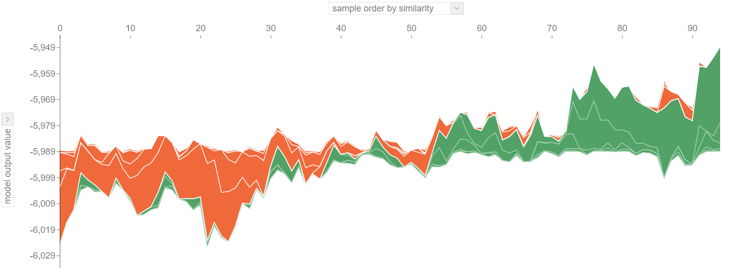
# Generate a SHAP force plot, and visualize the subtask predictions.
interpret.force_plot(X_train, y_train)
Example output (this plot is interactive in a notebook):
For additional examples, see the following directory.